Financial Modeling and Quantitative Analysis - Financial Modeling Software - Maple Features

Maple

Single User Licenses
Multi-User Licenses
Upgrade
What's New  |  Features  |  Online Demos  |  Compare  |  Training  |  Community  |  Free Trial  |  Buy Maple
Financial Modeling


Maple has many tools for advanced financial modeling, as well as accessible tools for personal finance.

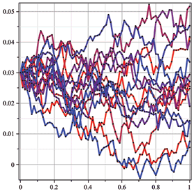
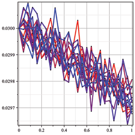
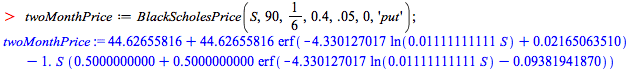
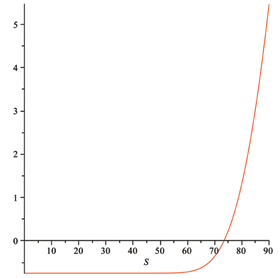
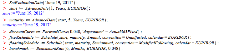
On the personal finance side, there are tools that can be used for computing with mortgages or retirement packages. The financial modeling tools include a wide range of stochastic processes that can be used to model option prices, such as Brownian motion, Ito processes, an SVJJ process, and more. It also includes tools to compose complex processes out of these building blocks. You can also create, manipulate, and analyze many types of financial instruments, such as American, Bermudan, and European options and swaptions and several types of bonds; short rate models; term structures of interest rates; and cash flows. The instruments can then be priced using analytic methods, lattice methods or Monte Carlo simulation - all using one of many date arithmetic conventions. Finally, the processes occurring in the package can be visualized in several ways.


Dig deeper:

Take a tour of the Finance Package
Explore an extensive collection of financial, time series data sets directly within Maple

financial modeling software

Personal finance

Annuities
If you would like to receive 100 units of money each year for 20 years (for, say, a retirement package), you need less than 2000 units to start with,because interest is paid (and compounds) over the sum that will be paid to you later. The amount needed can be computed by the annuity function. The following shows the result for an interest rate of 4%.


Interest formulas
Consider a loan of 100 units of money with a nominal annual interest rate of 4.5% where interest compounds every two months. The following command finds the accumulated value of the deposit over three years (that is, 18 periods).


The effective interest rate per year can be computed in the following two ways.


Stochastic processes

Many basic and more advanced stochastic processes are implemented in the Finance package. Here are a few examples.

Brownian Motion
A basic process is Brownian motion (with given initial value, drift, and diffusion).


Ito process

Ito processes are fairly general. Their drift and diffusion can depend on the state and time. For example, here is a process that gets much more volatile at
t = 2.


Heston process

A more advanced process is the Heston process, where the volatility is itself subject to a stochastic differential equation. This is implemented as a two-dimensional process.


You can see that some of the sample paths result in much higher volatility than others.

Composite process
Finally, you can compose multiple processes into one with a regime switching process, for example, for switching between two Brownian motion processes, one with high volatility and low drift and one with low volatility and high drift. The switching process is determined by a state transition matrix.


Interest rates

Term structures
The Finance package supports a number of different tools for interest rate term structures. You can define a yield curve in a number of different ways. This yield curve can be used to construct some of the more advanced short rate models described in the next section, or to compute zero rates, discount rates, or other similar rates.


Short rate models
The Finance package supports a number of different short rate models. The simplest is the Vasicek model.


The Cox-Ingersoll-Ross model is more advanced. It uses a yield curve.


Financial instruments: construction and pricing

Bonds

The Finance package supports bonds with a number of different types of coupons: zero coupon bonds, fixed coupon bonds, and floating rate bonds.


Get the set of cash flows for your bonds.


Calculate the clean price and the dirty price for your bond using the fixed rate of 5% as the discount rate.


Calculate the bond's yield using the previous discount rate.


Options
The Finance package supports American, European and Bermudan options with arbitrary payoff functions. The option is constructed separately from the process that describes the value of the underlying asset.
Consider a European strangle which pays off if the underlying asset deviates more than 20 units from 100, in either direction.

< img src="png/finance21.png" alt="" width="437" height="58" />


The option is priced using a Black-Scholes process for the underlying asset. The initial value is 100, the risk-free rate 5% and the volatility is constant at 40%. Assume no dividend is paid and divide the time from now to six months from now into 1000 equal time steps for lattice pricing.


You can also run a Monte Carlo pricing process.


Or, finally, compute the price analytically.


You can visualize the lattice and the Monte Carlo run together, but preferably using fewer time steps and replications. This time, a trinomial tree is used.


Here is a Bermudan put option with exercise times in four and six months and a strike price of 90.


Here is the lattice price.


Monte Carlo and analytical pricing are not built-in for non-European options. However, if you realize that after four months, the owner of the option can either exercise the option or she effectively now has a two-month European put option, you can still use this approach. Use the analytic approach to find the price of the European put option for two months if the current price is S:


As an aside, you can now determine at which value it is useful to exercise the put option after four months.


So if the current price after four months is less than crossover, the owner should exercise the option (she can always buy a European option for two months instead); otherwise, she should hold on to it. Either way, the value of the Bermudan option is the maximum of the exercise price and the price of the two month European option. Use this for a Monte Carlo simulation to find the current value of the Bermudan option.


Swaps and swaptions
Maple's Finance package can deal with interest rate swaps. You define the payment schedule and the type of interest rate.


Construct an interest rate swap with fixed rate 0 and compute the fair rate. This allows you to define the at-the-money rate for the at-the-money swap you will construct after that.


The swaption can be exercised from the day after the start of the swap, until the day after the one-but-last coupon payment date for the paying leg of the swap. These dates can be found as follows.


You can now price the swaption using lattice methods.


What happens if you take a finer or a coarser time grid? Let the number of steps vary between 50 and 1600.


The plot gives some confidence that further refining of the time grid will not change the first three significant digits.

Financial Modeling
Recorded Webinar


Learn about Maple’s unique set of features that make it ideal for financial modeling applications.


Watch the webinar